Welcome.

Overview of the course, its goals, target audience, necessary tools...

To be added.

Introduction to the PRESENT Cipher

If you’ve ever looked into cryptography for low-power devices, things like RFID tags, IoT sensors, or smart cards, then standard ciphers like AES can be overkill. They're secure, but they also demand more memory and processing power than some tiny devices can handle.

So comes PRESENT: a lightweight block cipher designed in 2007 specifically for environments where every byte and CPU cycle counts. It was proposed by researchers from Orange Labs and Ruhr-University Bochum, and is even standardized in ISO/IEC 29192-2.

From a cryptanalytic perspective, PRESENT is a great study case. It's a Substitution-Permutation Network (SPN), one of the most popular ways of constructing symmetric ciphers. In particular, its permutation layer is really simple in lieu of it needing to be fast, and is overall a cipher that's easy to imagine.

Over the next few lessons, we’ll use PRESENT to explore symmetric cryptanalysis methods like differential and linear cryptanalysis, and see what it takes to break (or at least weaken) a cipher.

Small cipher, big learning potential. Let's get started then: Hello World!!

Hello World!

To keep the course concise, we won't ask you to implement PRESENT from scratch (though you're welcome to do so!) and instead provide you with a finished implementation in TODO.

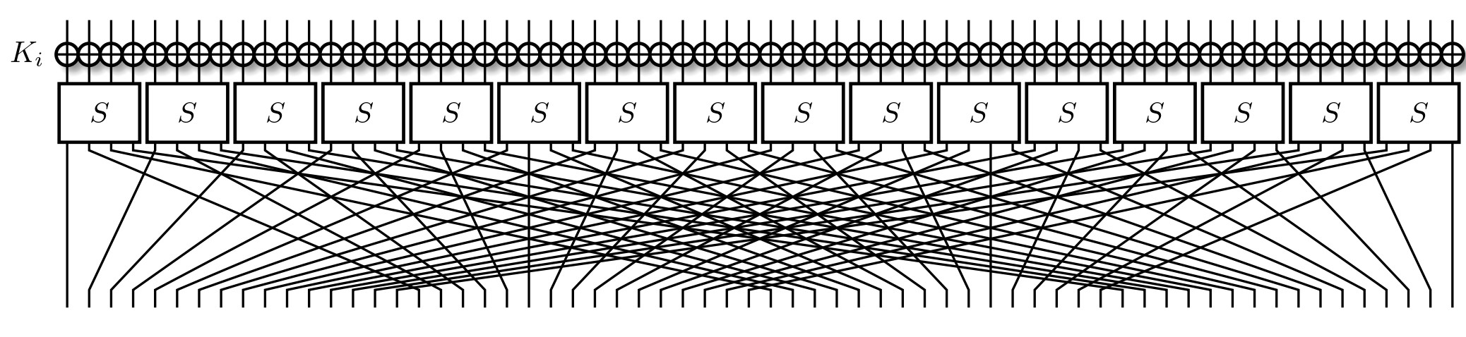
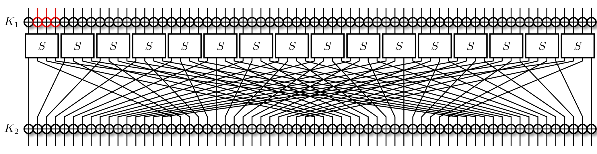
Traditionally, PRESENT has 32 rounds, with the last round being special. Like most SPNs, each round consists of three important aspects:

Round key addition: For each round, we XOR the state with the current round key.
Substitution: The state is subdivided into 4-bit chunks that're put through substitution boxes (S-Boxes). These are bijective maps: four bits go in, four come out.
Permutation: This is the linear layer of the cipher, responsible for mixing i.e. permuting the bits. It can be expressed as $f(x) = 16 * x \mod 63$, where $x = 0$ is the MSB. The LSB is special, and remains fixed.

A single round is pictured below.

One round of the PRESENT cipher

We did mention the last round being special. Unlike the others, it consists of only the round key addition.

Task: The last round of PRESENT does not include substitution and permutation after the key addition. Why?

That are two primary properties a symmetric cipher ought to have: confusion and diffusion. Confusion is the property that each output bit should depend on many input bits. This is a good thing, as the opposite makes the relationship between the ciphertext and key too obvious. This is accomplished via the prior mentioned S-Boxes, as each output bit is (partially) dependent on the four input bits.

The other is diffusion: the property that a slight change in the plaintext ought to influence a lot of the ciphertext, and vice versa. This is desirable because we don't want similar plaintexts to produce similar ciphertexts, and is accomplished via the permutation layer.

With that out of the way, let's try to decrypt a message. Using the key SYMMETRIC_CRYPTO, we've encrypted the following message with regular, 32-round PRESENT. Try to decrypt it, either with the provided implementation, or with your own.

0x823F2D4E3

Brute Force

The baseline of how strong a cipher, and what a cryptanalysist wishes to do better than, is an exhaustive search of the keyspace. In other words, any attack that is faster than simply enumerating all possible keys is considered a "cryptanalytic break" of the cipher. Whether such an attack is practical or not is a different story entirely.

PRESENT supports both 80-bit and 128-bits keys, which are then turned into thirty-two round keys using a key scheduling function. Right now, it's not too important how this function works, but more so the fact it exists. This means that despite the cipher consisting of thirty-two 64-bit round keys, its effective bit-security is only the size of the actual key. It should be noted that recovering the key is equivalent to recovering all round keys.

Despite this, it remains important to keep the way we generate our key important. To illustrate this point, we've encrypted a message with PRESENT. The key used was derived in the following way:

def random_roundkey(bits: int):
    t = randint(0, 2**bits)
    return int(sha256(str(t).encode()).hexdigest()[:16], 16)

cipher = Present(rounds=32, custom_roundkeys=[random_roundkey(20)]*32)

The ciphertext is TODO. Apply a brute force search to find a key, and decrypt the message.

Meet-in-the-middle

In the previous lesson, we made mention of a key schedule. Most ciphers have one, extending a single key into multiple, round-specific keys. The way PRESENT does this can be found in its specs. What matters right now is that each round has a different round key than any other, and the relationship between any two round keys is largely non-linear.

Obviously, a key schedule of some sort is needed; due to the block size (i.e. the input size) of PRESENT being only 64-bits, a static round key would imply a bit-security of 64 bits too, regardless of how we sample it from the main key. But why do we need different round keys for each and every round?

Suppose we instantiate PRESENT as follows:

def random_roundkey(bits: int):
    t = randint(0, 2**bits)
    return int(sha256(str(t).encode()).hexdigest()[:16], 16)

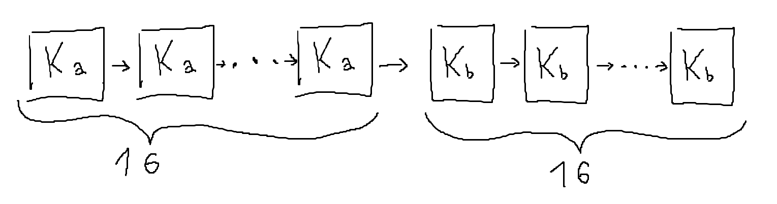
a, b = random_roundkey(20), random_roundkey(20)

cipher = Present(rounds=32, custom_roundkeys=[a] * 16 + [b] * 16)

Here we have two, 64-bit round keys. One can imagine this to be similar to a key schedule that'd simply split the key in two, and use those as our round keys. In our example, the first sixteen rounds use $K_a$ and the subsequent sixteen use $K_b$ as their round key. However, this proves almost no more secure than having simply used a static round key.

Meet-in-the-Middle

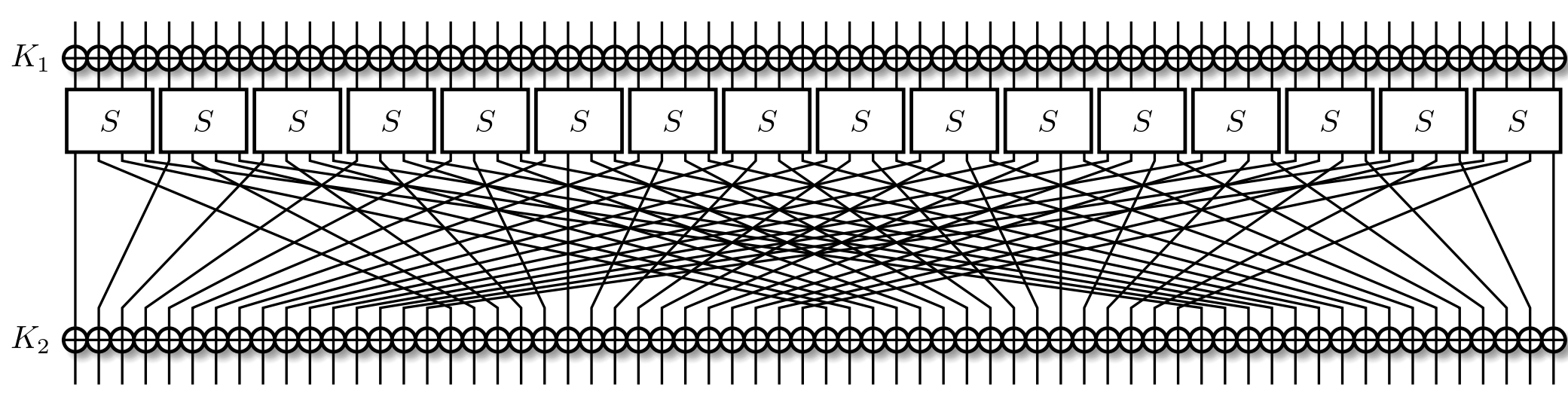
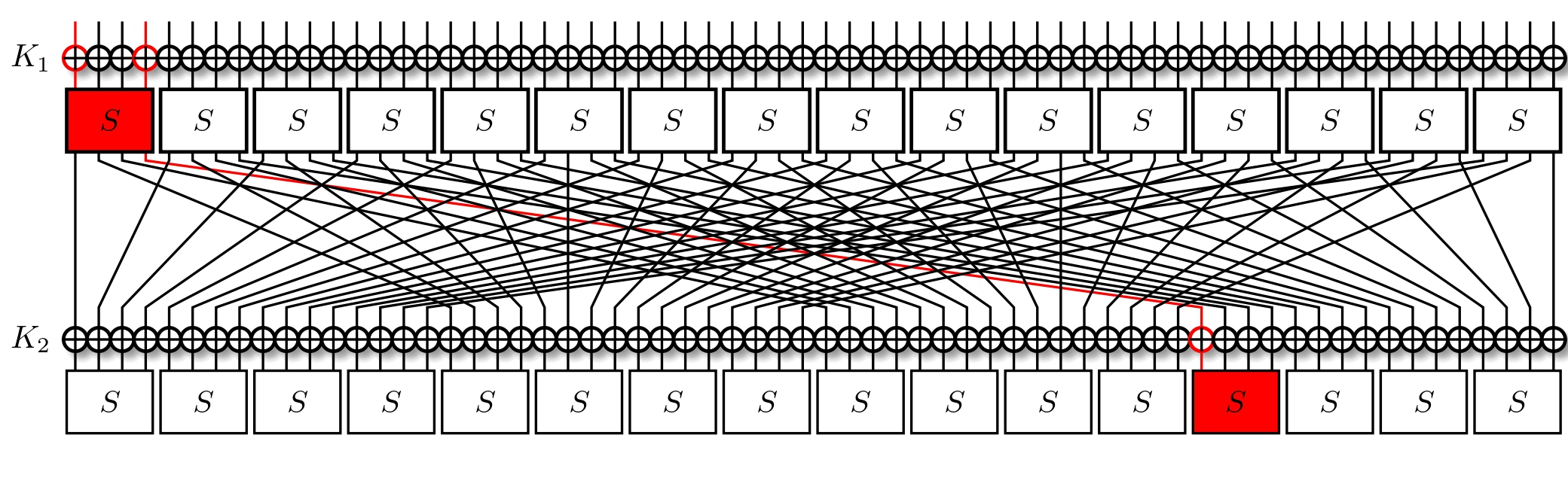
Let’s take a look at a tweaked version of PRESENT that just splits the master key $K$ into two, independent 64-bit round keys: $K_a$ for the first half of the cipher and $K_b$ for the second half.

Repeated keys of PRESENT

A naive approach would be to brute force both $K_a$ and $K_b$ and decrypt a ciphertext for each pair till the matching plaintext is produced. However, this proves incredibly slow: at two 64-bit round keys, it's a complexity of $2^{64} * 2^{64} = 2^{128}$, way beyond our (or anyone's) capabilities, and is just us guessing the entire key $K$.

Meet-in-the-middle (MITM) attacks are a way to do this more efficiently. The idea is simple: instead of attacking a cipher from one end, we attack it from both, starting from the plaintext side and the ciphertext side, and try to meet someplace in the middle. It’s a clever way to trade memory for speed, which can make brute-force-style attacks such as ours much more practical. The crux of the MITM paradigm is that we don't need to brute force both pairs at once, but that we can do so sequentially instead.

Here's how we'd attack this with a MITM approach:

Forward direction (plaintext $\rightarrow$ middle): For each possible value of $K_a$, run the first 16 rounds of the cipher starting from the plaintext $p$. That gives us an intermediate value $m$. We store all $2^{64}$ of these intermediate values in a table.
Backward direction (ciphertext $\rightarrow$ middle): Now, for each possible value of $K_b$, we run the last 16 rounds of the cipher in reverse, starting from the ciphertext $c$. For each partial decryption, we get a candidate intermediate value $m'$. Check if it shows up in the table of forward values from step 1.
Match found? If a match is found, we’ve probably got a good pair: one key that takes $p$ to $m$, and another that takes $c$ back to that same $m$. This gives us a likely $(K_a, K_b)$ pair.

This brings the time complexity down to about $2^{65}$: one full $2^{64}$ round of forward encryption, one full $2^{64}$ round of backward decryption. Much better than the $2^{128}$ we started with, and goes to show that using two round keys isn't all that great.

Of course, in our case, this comes with a memory trade-off. We have a memory complexity of $2^{64}$ due to storing all the intermediate values

Implement

Let's now write out an attack. Here's our cipher:

def random_roundkey(bits: int):
    t = randint(0, 2**bits)
    return int(sha256(str(t).encode()).hexdigest()[:16], 16)

cipher = Present(rounds=32, custom_roundkeys=[a] * 16 + [b] * 16)

Task Provided the following plaintext / ciphertext pair 059f909aa441d – 3f2341242d412 decrypt the following: 0x432fdffa11

Slide attacks

Earlier we discussed the situation where we use one round key for the first half of the cipher, and a different key for the second half. This setup allowed us to attack the cipher from "both sides". But what if we used the keys in an alternating fashion instead? Rather than using them for the first and second halves, we could use the keys one after the other like so:

def random_roundkey(bits: int):
    t = randint(0, 2**bits)
    return int(sha256(str(t).encode()).hexdigest()[:16], 16)

a, b = random_roundkey(BITS), random_roundkey(BITS)
cipher = Present(rounds=32, custom_roundkeys=[a, b] * 16)

Surprisingly, this proves not much safer, though for reasons that may not be immediately obvious. Before we dive into that, let's look at a simpler example:

def random_roundkey(bits: int):
    t = randint(0, 2**bits)
    return int(sha256(str(t).encode()).hexdigest()[:16], 16)

a = random_roundkey(BITS)
cipher = Present(rounds=32, custom_roundkeys=[a] * 32)

Till now, the best way we've seen to attack the cipher in such a setting has been brute forcing the round key as we did in 02 - Brute Force. This works well when the round key is small, say 32-bits or less, but a PRESENT round key is traditionally 64-bit. A natural question is whether there's a more clever way of abusing the lack of round key variety.

Visualising PRESENT

In 03 - MITM we split up the cipher into each of its rounds.

Repeated keys of PRESENT

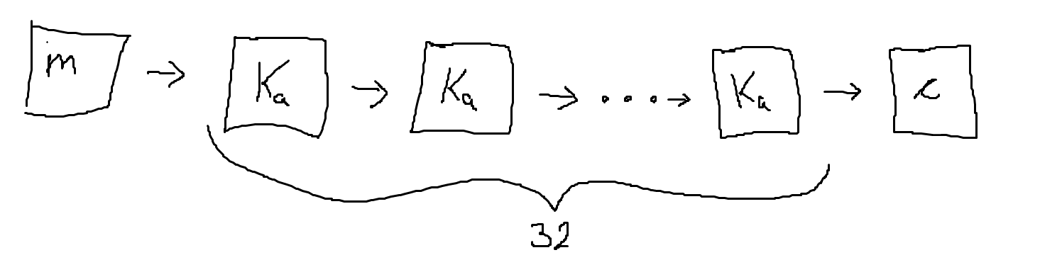
For a message $m$, after applying the 32 rounds of the cipher, we get a ciphertext $c$. Notice how each round is effectively the same function $f$ being applied consecutively. That is, $f^{32} (m) = c$.

Slid pairs

The block size of PRESENT is 64 bits. That is, both $m$ and $c$ are 64-bit values. Suppose we encrypt a large amount of messages. Then, by the birthday problem¹, we expect that after $2^{32}$ encryptions at least two of these ciphertexts should match. A similar argument tells us that we can expect to find two pairs $m_1$ and $m_2$ such that $c_2 = f(c_1)$. Were we to find such a pair (called a slid pair), we could attempt to find the round key — attacking just one round is much easier than thirty-two!

Earlier, we discussed what goes into a single round of PRESENT: key addition, substitution, and permutation. Out of these three operations, only the first is key dependent, meaning that the others can be inverted without knowing the key. This reduces process of finding the round key to a simple XOR operation!

Task 1 The following was encrypted with one round of PRESENT:
m = 0x14214213
c = 0x23123213
Determine the key.

In practice

Obviously, we can't check whether $c_2 = f(c_1)$ by just applying $f$ to ciphertexts because we don't know the round key. Instead, for every candidate slid pair (i.e. every pair), we attempt to recover the round key. Then we verify whether $f^{32}(m_1) = c_1$ for our recovered round key. If so, we've recovered the right one.

The other thing to note is that thus far we've been ignoring the last round of PRESENT; that is, we've been treating it as being no different than any other. Surprisingly, this isn't too much of a problem. As the last round is only missing the substitution and permutation steps, we can apply those two ourselves, and then continue with the assumption that all rounds are equal.

It's important to note that slide attacks are rather memory intensive. We need to store a lot of plaintext-ciphertext pairs. For a 64-bit blocksize, we anticipate $\approx 2^{32}$ blocks being needed, which comes out to about 34 gigabytes of storage. For larger block sizes, this quickly grows impractical as an approach.

The Slide Attack

Now it's your turn to implement the attack. The Wikipedia article may prove helpful.

Task 2 For the following slid pair, determine the key and decrypt the ciphertext 0x124324.

m1 = 0x123
c1 = 0x123
m2 = 0x123
c2 = 0x123

Task 3 Given the attached files, decrypt the ciphertext 0x123.

plaintext.txt

ciphertext.txt

The birthday problem, in the context of block collisions, tells us that for a $n$-bit blocksize we may expect a collision after $\frac{n}{2}$ blocks. ↩

Differentials

Previously, we talked about differentials. These refer to the differences in input and output for a simple passthrough of the S-Box. In practice, we're interested in how a differential propagates through multiple rounds of a cipher, all steps included.

To keep things simple, we'll only focus on finding distinguishers for now on. That is, ways to differentiate a cipher from random output. Later, we'll discuss how to turn distinguishers into key recoveries.

Following the differential

Let's focus on two-round PRESENT.

A normal round of PRESENT consists of a round key addition, the substitution, and then the permutation. We recall that in the last round, we only do the key addition part. This means, for 2-round PRESENT, our input is only going through an S-Box once, as seen below.

Since we care only about the differences in inputs and outputs, and the round keys are constant, we can safely ignore their impact on the differential. This should be rather clear as $$x \oplus y = (x \oplus K_a) \oplus (y \oplus K_a)$$

We've discussed the S-Box already. We have a differential and are running on the pretense that a certain difference will hold with a certain probability that we can distinguish. What remains to be seen is how this differential scatters due to the permutation layer. Let's reuse our example from earlier, and suppose we have $\Delta_{\text{in}} = 7$. To simplify our discussion, we will use $x_0, x_1,\ldots , x_{15}$ to denote the intermediate difference in each step. The values $x_0, x_1,\ldots , x_{15}$ are 16 nibble differences, with $x_0$ being the least significant nibble difference.

Let's place our input difference in the most significant nibble, i.e. let $x_{15} = \Delta_{\text{in}} = 7$.

We'll reuse the differential $7 \rightarrow 1$ from the previous lesson. Post-substitution, we then have that $x_{15} = 1$. This is then permuted by the next layer, and then the second round key addition occurs. Following the permutation, we have that $x_{3} = 8$.

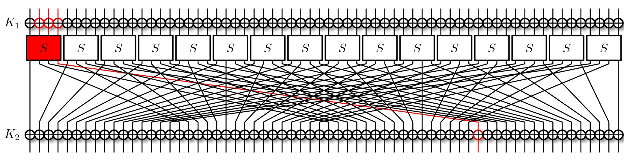
Recall that the probability that this differential holds is $p = \frac{4}{16} = 0.25$. This implies that we can expect that, for one out of every four input pairs, the corresponding output pairs will differ by exactly $x_{3} = 8$ with all else being the same. Formally, for our two rounds, we can say that $$ \text{Pr}[\text{Enc}(x\oplus \text{(0x7 $\ll$ 60)}) = \text{Enc}(x) \oplus \text{(0x8 $\ll$ 12)}] = 0.25 $$

With this, we have traced our differential. It's now natural to be curious whether we can extend it.

Distinguishing from random

Now that we have a differential, it remains to be seen how useful it really is. What does it mean for us to have a difference in the output, and how can we use this?

The procedure for exploiting a differential would be as follows:

Find a differential $x \rightarrow y$ that holds with a probability $p$
Generate a random input $r$ and encrypt $(r, r \oplus x$)
For an output $(c_1, c_2)$ check whether $c_1 \oplus c_2 = y$. Repeat this many times, and estimate how often it holds

If our outputs exhibit a differential property largely in line with how often we expect it too, then it's likely that we're dealing with real ciphertext. Otherwise, it could be just random data. Note that random data, assuming a 64-bit block size, can exhibit any difference with a probability of $2^{-64}$. This is what we're trying to beat with our own differentials.

Differentials that enable us to distinguish ciphertext from random data are called differential distinguishers. Later we'll see how we can push this further, and recover a key. But first, we'll look at how we can get more meaningful ones.

Differential trails

We've talked about finding a differential, and how to use one. However, we've barely attacked PRESENT thus far. For a cipher with 32 rounds, tackling just two (really, it was one and a half) seems silly. This is what we seek to address with this section.

Recall that a differential is the observed difference following an S-Box. We define a differential trail as our set of differences as we follow a differential through the cipher. Sometimes this is referred to as a differential characteristic instead. Some authors may make a distinction between the two terms. For simplicity, both mean the same thing to us.

Trails

Previously, we actually used the differential $7 \rightarrow 1$ to make a rather basic trail. Traditionally, trails are noted by making a note of the entire state as follows, arrows connecting rounds. $$\text{0x7} \ll 60 \rightarrow \text{0x8} \ll 12$$ As this isn't helpful when constructing these trails on our own, and does little to really show what the impact of the permutation layer is, we will use the following notation for the duration of the course: $$ \begin{array}{|c|c|c|c|} \hline \text{Round} & & \text{Differences} & \Pr \ \hline \text{I} & & x_{15} = 7 & 1 \ \hline \text{R1} & S & x_{15} = 1 & 2^{-2} \ \hline \text{R1} & P & x_{3} = 8 & 1 \ \hline \end{array} $$

The second column denotes the layer of the round. We ignore the key addition step for brevity as it has no impact on the difference. The last column denotes the probability of our difference holding. The total probability of a differential trail is the product of all its differentials' probabilities.

This isn't a particularly impressive trail as it spans more than one round only by technicality, but it lays the groundwork for what we want to achieve. From now on, we'll be looking at the real deal: 32-round PRESENT. It's worth noting that if we find a trail that spans, say, four normal rounds, it effectively works on a 5-round variant of PRESENT.

Continuing our trail

We left off at $x_{3} = 8$, so we need to look at what new differential to add onto our trail. For this, we consult our DDT, looking at the row for $\Delta_{\text{in}} = 8$:

  Δ  0 1 2 3 4 5 6 7 8 9 a b c d e f
------------------------------------
8 |  0 0 0 2 0 0 0 2 0 2 0 4 0 2 0 4

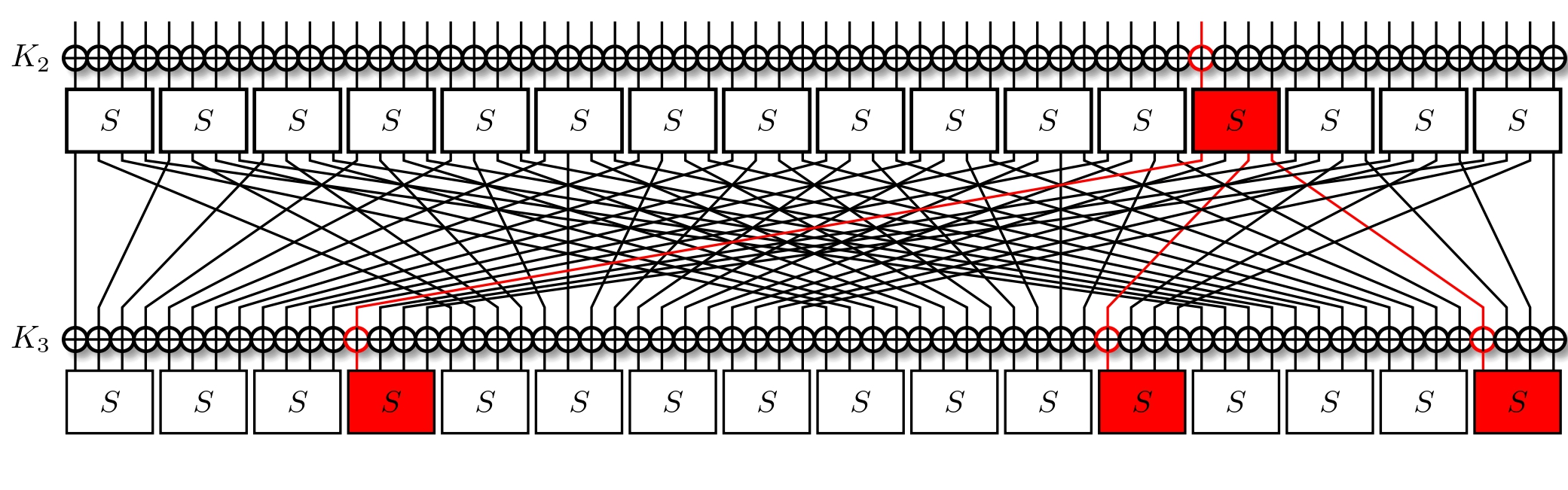
Recall that it's in our interest to pick differentials with high probability of occurrence. We'll go with the choice of $8 \rightarrow \text{b}$ for our next differential, once more holding with probability $0.25$. We now have that $$ \begin{array}{|c|c|c|c|} \hline \text{Round} & & \text{Differences} & \Pr \ \hline \text{I} & & x_{15} = 7 & 1 \ \hline \text{R1} & S & x_{15} = 1 & 2^{-2} \ \hline \text{R1} & P & x_{3} = 8 & 1 \ \hline \text{R2} & S & x_{3} = \text{b} & 2^{-2} \ \hline \text{R2} & P & x_{4} = 8, x_{11}=8, x_{15}=8 & 1 \ \hline \end{array} $$ Note that our differential is now seen in three bits as $\text{0xb} = \text{0b1011}$. From this, due to the permutation, we will have up to three S-Boxes active in the second round. In fact, we have exactly three.

trail

We now have a two-round differential trail that holds with a total probability of $2^{-2} * 2^{-2} = 2^{-4}$. It seems to be going well, but what determines if a trail is good? And what is our goal?

Good differential trails

Active S-Boxes are traditionally something we'd like to minimise as an attacker, and maximise as a designer. The so-called branch number $\mathcal{B}$ for a cipher tells us what the minimal amount of active S-Boxes is for any two consecutive rounds. The lowest it can be is obviously $\mathcal{B} = 2$. Meanwhile, the most it can be for a SPN is $\mathcal{B} = 1 + \text{no. of S-Boxes per round}$ as the first round could only have one S-Box active.

It's not hard to imagine, and in fact is fun to find, the differential trail for PRESENT by which only two S-Boxes would be active in the first two rounds. Finding it is how we may prove that PRESENT has a branch number of two. This can be considered bad in comparison to e.g. AES, which has a branch number of five, but enough rounds can supplant the issue.

Task Find a differential trail which proves that the $\mathcal{B} = 2$ holds for PRESENT. Additionally, find a trail that proves the branch number for three consecutive rounds is $3$.

Theoretical security

Branch numbers are useful as they tell us how many rounds we should aim to have. The PRESENT cipher has a branch number of 2, and a differential uniformity of 4. This means that the minimum amount of active S-Boxes corresponds to the number of rounds, and the maximum probability of a differential per S-Box is $2^{-2}$. This implies that, for its 32 rounds, the best possible differential trail holds with a probability of $({2^{-2}})^{31} = 2^{-62}$. For comparison, a trail wants to hold with a probability better than "random", i.e. the probability of a pair of blocks differing by a desired amount (which is equal to $2^{-64}$ for to the block size of PRESENT).

This above may sound worrying. It is, after all, an argument made that lends belief that PRESENT is weak to differentials. However, in the specification of the cipher, the designers go on to prove that PRESENT's branch number for five consecutive rounds is 10, so for 25 rounds there will be at least 50 active S-Boxes. This is much better than our earlier assumption, and leads to standard differentials trails having a probability of less than $2^{-100}$ over all the rounds.

Finding trails

Previously, we went over what a differential trail is, and how they're made. Now we will go over how to find and exploit them. This is going to be a more coding-heavy section, and mostly involves automating the tiresome process of before. There's no harm in skipping this section, though it can be quite useful to know.

Matsui's algorithm

For a while, Matsui's branch-and-bound trail search algorithm was favored and continuously refined by the cryptographic community. At present, the method has been largely supplanted by more powerful ones, so we include this section out of historical interest. However, it's still a fundamental and is simple enough to offer insight into how to find good trails quick.

The idea is rooted in what we discussed earlier regarding differential uniformity and branch numbers. Suppose we have a differential that holds with probability $p$ over $r$ rounds and we're interested in finding a better one. For simplicity, we'll assume a fixed starting difference as well. What we can do is as follows:

We branch. For every active S-Box, we iterate over possible output differences based on our input difference. We then propagate these differences via the linear layer.
We bound. The differences are assumed to propagate ideally through the rest of the cipher (based on our differential uniformity and branch number). This is then compared to our current best result. If it's worse, we prune this difference.
If a trail reaches the end without being pruned, it's saved as a good trail

What's interesting is that Matsui's algorithm can be considered exhaustive, making it great for smaller ciphers. It can also be used to e.g. estimate a branch number for a larger number of consecutive rounds.

Task Using Matsui's algorithm, find the best differential trail for 3-round PRESENT.

Task Using a modified version of Matsui's algorithm, find the branch number for three consecutive rounds of PRESENT.

Automated searching

As mentioned prior, Matsui's algorithm is no longer the state-of-the-art. More processing power and algorithmic improvements have made more generic optimisational problem-solvers the future.

MILP (Mixed Integer Linear Programming) is a powerful method that can be used for automating the search for differential trails in block ciphers. Instead of manually exploring the trail space (as in Matsui’s branch-and-bound algorithm), MILP models the cipher's behavior as a set of linear constraints and uses an optimisational solver to find trails of maximised probability.

For this section, we use PuLP, a Python library that abstracts MILP modeling. It supports many popular MILP solvers like CBC, Gurobi, and CPLEX.

S-Box modelling

As mentioned, MILP solves optimisational problems expressed as linear systems. In our case, we want to maximally increase the probability that a differential holds, which means maximising the weight of a differential trail. Because we're dealing with only linear systems, we do have to get clever with how we model these things.

There is an assumed familiarity with Mixed Integer Programming here. In case this is new to you, head over to the optional section Intro to MILP where we first go over a simpler example and explain the basics of how MILP works.

That out of the way, let's start with just one round. For ease, we'll represent the input and output as 64 binary variables.

import pulp

model = pulp.LpProblem("PRESENT", pulp.LpMaximize)
x = [pulp.LpVariable(f"x{i}", cat='Binary') for i in range(64)]
y = [pulp.LpVariable(f"y{i}", cat='Binary') for i in range(64)]

Now we model the S-Boxes. We will need to reuse the values from our DDT from earlier so that we can account for the differentials.

selectors_per_sbox = []
for sbox in range(16):
	selectors = []
	for in_diff in range(16):
		for out_diff in range(16):
			weight = DDT[in_diff][out_diff]
			if weight == 0: # Ignore impossible differentials
				continue
			sel = pulp.LpVariable(f"sel{sbox}_{in_diff}_{out_diff}", cat='Binary')
			selectors.append((sel, in_diff, out_diff, weight))
	selectors_per_sbox.append(selectors)

The selectors are binary values just as well. A one indicates that the differential is active. We don't necessarily want to minimise the amount of active bits or differentials, but we do want there to be at least one (and, if counting the trivial differential, exactly one for each S-Box). We also don't want our differentials to be invalid — a differential should only be considered if the input bits permit it. So we now fix that.

total_weight = []

def nibble_extr(bits):
    return sum(bits[i] * (1 << (3-i)) for i in range(4))

for sbox in range(16):
	selectors = selectors_per_sbox[sbox]
	in_bits = x[sbox*4:(sbox+1)*4]
    out_bits = y[sbox*4:(sbox+1)*4]
    dx = nibble_extr(in_bits)
    dy = nibble_extr(out_bits)
	
	# Exactly one differential per S-Box
	model += pulp.lpSum(sel for sel, _, _, _ in selectors) == 1
	# The input bits the differential wants must match the actual input bits  
	model += dx == pulp.lpSum(sel * diff_in for sel, diff_in, _, _ in selectors)
	# Likewise for the output bits
	model += dy == pulp.lpSum(sel * diff_out for sel, _, diff_out, _ in selectors)
	# We keep a track of our active weights, i.e. probabilities
	total_weight += [sel * w for sel, _, _, w in selectors]

All that's left now is to model the permutation, add our function, and see where our best differentials ended up.

y_perm = [pulp.LpVariable(f"y{i}_perm", cat="Binary") for i in range(64)]
for i in range(64):
    model += y_perm[PBOX[i]] == y[i]

model += pulp.lpSum(total_weight)
model.solve()

We've got a single round of PRESENT modelled now. This is actually quite useful on its own. Were we to ever get "stuck" with a differential, we could extend it by one round by just fixing some of the input variables. Expanding the above to work for more rounds isn't as hard, though it will involve more variables. As the number of variables, and inherently the number of equalities, increase, so does the complexity of solving.

Task The above code can be said to "work", but only by technicality: it outputs the trivial differential as the best one. Add a constraint such that the trivial differential isn't always the best one. This can also be done by excluding it as a selectable differential, but then you'll have to change the constraint forcing every S-Box to be active.

More rounds

Now it's on you. One round is good, but we can do better than that. This is done best by adding more variables, and mapping old ones to new ones after each round.

Task Expand the above code to analyse four rounds of PRESENT.

Key recovery

A distinguisher is only half the story. Let's go after the key.

Turning distinguishers into keys

Fundamentally, a distinguisher tells us that a cipher exhibits a distinguishable property after $n$ rounds. On its own, this can be useful for e.g. telling apart cipher encryption from random output. More interestingly, this can be used to mount a key recovery attack.

The idea is founded in the fact that the specifics of the distinguisher change from round to round. If we could guess the last round key, we could easily reverse the last round and verify whether the distinguisher holds.

In many ciphers, retrieving a single round key is as good as retrieving the entire key. Intuitively, this makes sense: for an $n$-bit key, we have $n$ bits of entropy in the entire cipher. Were it not so, it would imply the round keys to be quite weak.

Reversing a round

For a cipher with $n$ rounds, the idea is as follows.

Find a $n-1$ round distinguisher and identify the active bits
Guess bits of the round key so as to reverse the final round and note the active bits
If the distinguisher holds with notable probability, the guessed bits are the actual bits

Sometimes, we can recover a good chunk of the round key by doing so, but not enough that a brute force for the remaining bits is feasible. In such cases, we look for a new differential trail, and apply it, slowly recovering the entire key.

TODO: Remote task here. Idea: low rounds with limited queries to force good differentials, repeated round key

Linear cryptanalysis

Linear cryptanalysis is, alongiside differential cryptanalysis, one of the most fundamental forms of cryptanalytic attack against symmetric block ciphers. Like differential cryptanalysis, it too is rooted in the statistical analysis of the cipher. Unlike it, though, it is a known-plaintext attack. We don't need access to an oracle to abuse it, only a lot of messages.

Originally introduced by Mitsuru Matsui in the early 1990s, this technique was used to mount the first known attack on the full 16 rounds of the Digital Encryption Standard (DES). Since then, it has become a cornerstone of cipher evaluation and design.

Here we'll go over the core ideas behind linear cryptanalysis: what it means to "approximate" a cipher with linear expressions, how we measure the quality of these approximations, and why (and how!) they can be exploited.

Linear Cryptanalysis

At its heart, linear cryptanalysis tries to find linear relationships between the input bits, output bits, and key bits of a cipher. In other words, we're interested in approximating nonlinear functions with linear ones. These relationships usually don’t hold always, and instead with some probability. If this probability is significantly different from 0.5 (i.e. very different from a random permutation, i.e. "biased"), we can use that bias to infer information about the key.

Somewhat more formally, the cryptanalyst's goal is to find Boolean expressions of the form:

$$P_i \oplus P_j \oplus \cdots \oplus C_k \oplus C_l \oplus \cdots = K_m \oplus \cdots$$

that hold with probability $p \neq \frac{1}{2}$, where:

$P$: bits of the plaintext,
$C$: bits of the ciphertext,
$K$: bits of the key.

A truly random permutation (which is a cipher's goal to emulate) should have such expressions hold with probability exactly 0.5. Any consistent deviation can tell us something about the key.

Bias

A central idea in linear cryptanalysis is bias: the amount by which a linear approximation deviates from $\frac{1}{2}$. It can be understood as how dependable our approximation is. We calculate it as $p - \frac{1}{2}$ for a probability $p$, so it is bounded by $[-\frac{1}{2}, \frac{1}{2}]$. The greater the magnitude, the greater the bias; we want to get as far away from zero as possible.

Formally put, let $X$ be the function of some bits of the plaintext and ciphertext (and possibly the key), and $q$ a linear approximation of $X$. We define the bias $\varepsilon$ as: $$\varepsilon = \Pr[X = q] - \frac{1}{2}$$ The larger the absolute bias $|\varepsilon|$, the more useful the approximation. This may be counter intuitive at the moment, but a relation that's almost never holds is as useful as one that almost always holds; approximations that're no better than guesswork are what we seek to avoid. Even a small bias (e.g., $\varepsilon = 2^{-10}$) can be exploited with enough data, as we'll see later.

Correlation

For practical reasons, we prefer the bounds of our bias to be "nicer". Doubling the bias, we get the correlation for a given approximation. That is, we define $$ \textbf{corr} = 2\epsilon $$ Our correlation is then bounded by $[-1, 1]$. This comes with a lot of benefits we'll only see later. For now, we'll try to express everything in terms of correlation.

Approximating Basic Boolean Functions

Before we get to approximating an S-Box, it’s helpful to see how we approximate basic Boolean operations like AND, OR, and XOR. These approximations lay the groundwork for understanding how nonlinear components can be approximated with linear expressions.

Approximating XOR

Let’s start with the easy one. The XOR operation is already linear (over $\mathtt{F}_2$), so it doesn't need approximation: $$x \oplus y = x + y \mod 2$$ Finding linear combinations of bits via XOR'ing them (e.g. $x_1 \oplus x_2 \oplus x_5$) is exactly what we’re trying to use in linear cryptanalysis.

Approximating AND

The AND operation, however, is not linear. Consider the table:

$x$	$y$	$x \land y$
0	0	0
0	1	0
1	0	0
1	1	1

We want to approximate this function with something linear (a XOR of input/output bits). One good approximation is simply: $$x \land y \approx x$$ This approximation is obviously correct if $y = 1$, which happens half the time (assuming random inputs), and is also correct whenever $x = 0$. In total, this approximation is correct 3 out of 4 times. So:

$\Pr[f(x, y) = x] = \frac{3}{4}$
Bias $\varepsilon = \frac{3}{4} - \frac{1}{2} = \frac{1}{4}$
Correlation $\textbf{corr} = 2\epsilon = \frac{1}{2}$ This isn't the only (good) approximation though. Other possible approximations are:
$x \land y \approx y$ (same bias),
$x \land y \approx 0$ (correct in 3 out of 4 cases as well)

Approximating OR

Another common Boolean function is OR, which is also nonlinear. We know that the OR operation behaves as follows:

$x$	$y$	$x \lor y$
0	0	0
0	1	0
1	0	0
1	1	1

Immediately, we can spot several good approximations. The obvious one is $x \lor y \approx 0$, while a more interesting one is $x \oplus y$, both holding in 3 of out of 4 cases. This then gives us a bias of $\varepsilon = \frac{1}{4}$, and a correlation of $\textbf{corr} = \frac{1}{2}$.

Task Both OR and AND don't actually have "bad" approximations. That is, neither has a linear approximation that has a bias of $\varepsilon = 0$, and the absolute bias for every approximation is always $|\varepsilon| = \frac{1}{2}$. Using the basic properties of linear functions, prove this claim.

Why this matters

S-boxes are just small Boolean functions. In PRESENT's case we've 4 bits going in, and 4 bits coming out. Internally, they’re implemented using combinations of AND, OR, XOR, and NOT. We've shown the first two to be nonlinear, while the last two certainly are linear. In the next section, we'll create a Linear Approximation Table (LAT), by which we’re measuring how well we can approximate more complex Boolean functions (such as an S-Box) with XOR expressions, just as we did above.

The above understanding of biases in basic gates helps us appreciate where the approximations in the S-box come from, and why certain input/output combinations are more useful than others.

Linear approximation table

Masks

Before we proceed with analysing an S-Box, we need a more concise and practical way of writing down linear approximations. This is the role of a (linear) mask.

Formally, suppose we have a Boolean function that takes as input an $n$-bit input vector $(x_0, \ldots, x_{n-1})$. We define a mask $\alpha = (\alpha_0, \ldots, \alpha_{n-1})$ as an $n$-bit vector such that each $\alpha_i \in {0,1}$. More often, we'll be interested in the dot product of the mask and the vector, expressed as: $$\alpha \cdot x = \bigoplus_{i=0}^{n-1} \alpha_i x_i$$ A mask just isolates which bits we consider "active", discarding the rest. Programmatically, it is the Boolean vector by which we may AND our vector.

As an example, the input and output masks $\alpha = {0, 0, 1, 0}$ and $\beta = {1,0,1,1}$ for a 4-bit Boolean function (e.g. PRESENT's S-Box) represent the following approximation: $$ x_2 = y_0 \oplus y_2 \oplus y_3 $$

The LAT

Thus far, we've been using bias and correlation to estimate our approximations, preferring it over raw probability. All of these stem from a more fundamental expression: the number of solutions, which is just for how many cases does the approximation hold for.

For a Boolean function $f$, a given input mask $\alpha$ and output mask $\beta$, we can formally write down the bias as $$\varepsilon_{\alpha, \beta} = \Pr[\alpha \cdot x = \beta \cdot f(x)] - \frac{1}{2}$$ and with $s$ we label the total number of solutions (i.e. inputs) for which the equality holds. $$ s = #{x\ |\ \alpha \cdot x = \beta \cdot f(x) } $$ One idea for representing the linearity of an S-Box may be to simply list out the total count of solutions. We prefer not to do this as, among other reasons, it doesn't capture the idea that an approximation having few solutions is as good as one having many. Instead, we have 0 be the worst i.e. random approximation, and have our "good" values go into the positives, and our "bad" values into the negatives. That is, we center our values around the expected average. This'll be made clear in a moment.

Similar to the Difference Distribution Table (DDT) for differential cryptanalysis, we now define the Linear Approximation Table (LAT) for linear cryptanalysis. The formula for computing it is $$ \text{LAT}[\alpha][\beta] = s - 2^{n-1} = 2^n \epsilon = 2^{n-1}\textbf{corr} $$ where $n$ is the input size of our Boolean function (in the case of PRESENT's S-Box, $n = 4$). Visually, this would look like the following:

α\β   0  1  2  3  4  5  6  7  8  9  a  b  c  d  e  f
...
7 |  0  0  0  4  4  0  0  0  0 -4  0  0  0  0  4  0 
8 |  0  0  2 -2  0  0 -2  2 -2  2  0  0 -2  2  4  4 
...

Zero entries correspond to mask pairs that behave as a random function (i.e. aren't biased), so we only care about the non-zero values.

Task Generate a LAT for the S-Box of PRESENT, complementing the above output. You'll need it for later.

The LAT has some interesting properties at a glance. The most glaring is that every value is even. This makes sense if we take time to think about it. Each possible input $x$ for some mask either holds and increases the value, or doesn't hold and decreases the value. If the total amount of inputs is even (which it is, being $2^n$) then every entry must be even.

Sometimes (although not in the case of PRESENT), an S-Box may have an "ideal" approximation, i.e. some approximations always (or very frequently) hold. These are called (perfect) linear structures. As they aren't observable in PRESENT, we will be ignoring them for now, and mention them only for completeness sake.

Task In linear cryptanalysis, we're often more concerned about correlation than anything else. Rather than displaying the number of solutions, display the correlation that any given approximation holds. This is called a correlation table.

Linear trails

Thus far, we've kept using bias (and correlation). It may seem tempting to rely on probabilities when discussing approximations. However, this has a few shortcomings which we will now go over, and improve upon.

Distinguishers

Much like with differential cryptanalysis, the focus of our attacks is on preparing distinguishers — that is, a way to differentiate a cipher's output from random output. This is actually what we've been buildings towards this entire section. By using and verifying our approximations, we can tell whether we're dealing with a biased output quite easily. The only question that remains is how to do so efficiently.

Let's tackle the PRESENT cipher again, specifically its first round. We'll pick out some initial mask $\alpha = 9$ for the input of the top-most S-Box. The XOR is linear, and so doesn't change what bits we're observing.

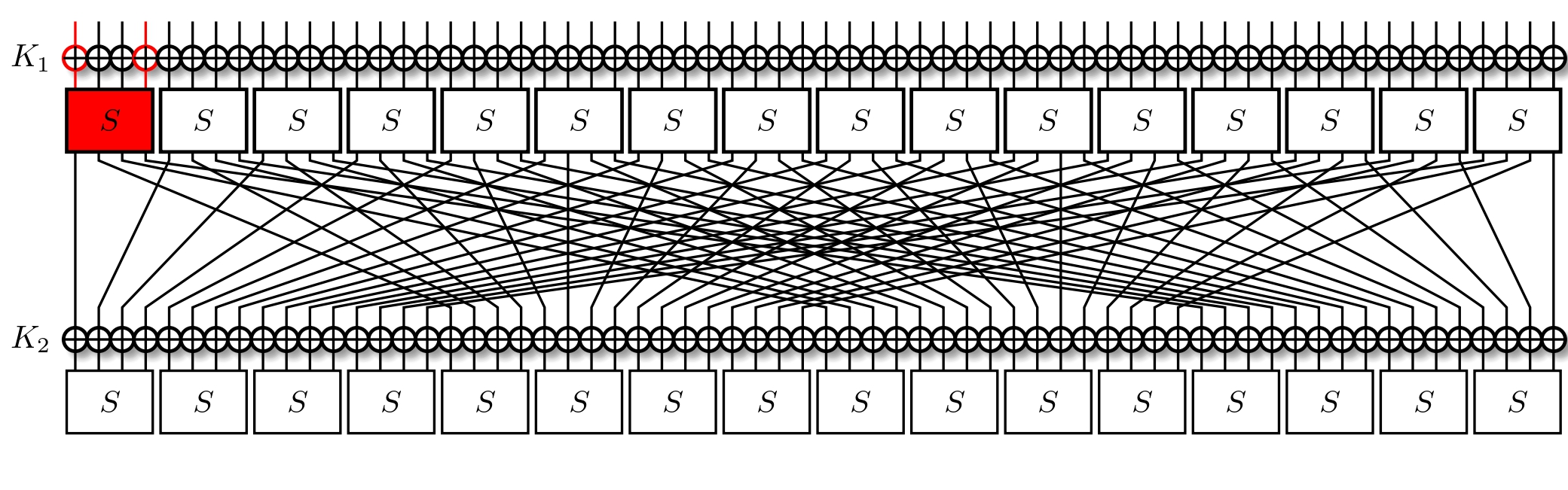
PRESENT with its leftmost S-Box active

We now check the LAT, and see which output masks have with a bias. We take $\beta = 1$ as our example; it holds for $\text{LAT}[\alpha][\beta] = 4$ inputs more than expected, so with a probability of $p_1 = \frac{12}{16}$ and with a bias of $\epsilon_1 = p - \frac{1}{2} = \frac{1}{4} = 2^{-2}$ ($\textbf{corr}_1 = 2^{-1}$). For one round, this is simple to calculate and use: we have the expected probability right there. But how does the situation evolve when we go for a second round?

The chosen output mask results in one active bit. We follow this bit through the permutation layer, and find it ending up in another S-Box.

Activation of the second substituton layer of PRESENT

This time around, we have $\alpha = 8$, so we consult our LAT. A strong approximation would be $\beta = \text{0xe}$, holding in $\text{LAT}[\alpha][\beta] = 4$ inputs more than were it a random approximation. So it holds with probability $p_2 = \frac{12}{16}$ and a bias of $\epsilon_2 = p - \frac{1}{2} = 2^{-2}$ ($\textbf{corr}_2 = 2^{-1}$).

How do we know the overall, 2-round probability? One idea may be to simply multiply the probabilities. After all, it is what we did for differential trails. However, this doesn't really work, and it may not be obvious why not either.

Issues with probability

Starting off, the two approximations we made are not independent events, meaning that they cannot be multiplied so simply. In fact, even the first substitution is not quite what we make it out to be. While we easily ignored the round-key additions during differentials, we cannot do so for linear approximations. If a key-bit is 0, the bias remains the same. If a key bit is 1, it changes its sign. Meaning that the probability that it holds flips just as well.

This can also be seen from our earlier definition of the solution space: $$ s = #{x\ |\ \alpha \cdot x = \beta \cdot f(x) } $$ Accounting for key-addition, we have that: $$ s = #{x\ |\ \alpha \cdot (x \oplus k) = \beta \cdot f(x) } $$ Since we only care about the inner product, a single bit change also changes when we have an equality.

This all implies that any key-addition affects the probability. However, it doesn't impact the bias that much- more specifically, it doesn't impact the magnitude of it, only the sign. This is why we introduced and use bias and correlation; they remains relevant round after round.

Piling-up lemma

As it turns out, we have a nice instrument by which we can combine multiple consecutive approximations. We state the following lemma:

Piling-Up Lemma: Suppose $T_i$ are independent discrete random variables with correlations $\textbf{corr}_j$, $j=1,2,\ldots,k$. Then the correlation $\textbf{corr}$ of $T = T_1 \oplus T_2 \oplus \ldots T_k$ can be calculated as $$ \textbf{corr} = \textbf{corr}_1 \textbf{corr}_2 \cdots\textbf{corr}_k$$

The above can be restated with bias as well, but is less clear. The proof for the lemma is usually done via induction and using biases, and we omit it for brevity, but it can be found in e.g. these slides.

The impact of the lemma is that we can simply multiply the correlations to get our total correlation. This is much simpler to work with, and what we'll be going with forwards. In the next section, we'll look at extending this trail further, and then using it to attack the cipher.

Approximations in practice

Enough theory. Let's get our hands dirty.

Extending the trail

We'd looked over a two-round trail on PRESENT, but we didn't properly try to exploit it. Recall that the an advantage of linear cryptanalysis is that we aren't reliant on choosing our messages, and are operating in a known-plaintext model.

Our two-round approximation was $\text{0x9} \ll 60 \rightarrow \text{0x8} \ll 12$, meaning we're currently at the following step:

PRESENT with one S-Box active

It's important to recall that we're trying to minimise the number of active S-Boxes. This usually means that we're trying to also minimise the number of active bits, all the while maximising the correlation. Taking a look at the LAT, we find that for an input mask of $\text{0x8}$ we've two output masks with a correlation of $2^{-1}$, those being $\text{0xe}$ and $\text{0xf}$. Out of these, the former activates less bits, so we opt for it instead. With three active bits, we trace them through the permutation layer, and now activate three S-Boxes.

PRESENT with 3 active S-Boxes on the next layer

Notice how we have the same input masks in all three S-Boxes? What's more, they're the same that we used for the previous layer. To simplify, we can just reuse our previous approximation, and watch it propagate.

Following the XORs of the 3 S-Boxes

We're interested in the overall correlation. Recall that it's equal to just the product of all of our approximations. So total correlation of above output masks for the initial input mask of $\text{0x3} \ll 60$ is $$ \textbf{corr} = \textbf{corr}_1\textbf{corr}_2 \textbf{corr}_3 $$ equating to $$ \textbf{corr} = 2^{-1}2^{-1}(2^{-1})^{3} = 2^{-5} $$ To notice a correlation $\textbf{corr}$ with a bias $\epsilon$ we need $N$ plaintext-ciphertext pairs, where $N$ is $$ N \approx \frac{1}{\epsilon^2} = \frac{4}{\textbf{corr}^2} $$ Naturally, this can vary for a lot of reasons, but in general we expect it to hold. In our case, we expect to need $N \approx 2^{12}$ pairs to notice the approximation.

Now we collect many plaintext-ciphertext pairs for 4-round PRESENT, and observe whether the XOR of the input bits and output bits is equal.

cipher = Present(key=randbytes(16), rounds=4)

inmask = 0
for i in [0,3]:
    inmask ^= 1 << (63-i)

outmask = 0
for i in [3,7,11,19,23,27,35,39,43]:
    outmask ^= 1 << (63-i)
  
pts = []
cts = []

N = 2**12
for _ in range(N):
	pt = randbytes(8)
	ct = cipher.encrypt(pt)
	pts.append(int(pt.hex(),16))
	cts.append(int(ct.hex(),16))

Recall that we expect a XOR of random variables to be similar to a random distribution, so it's best to compare these results to one.

def xorsum(value):
    xorsum = 0
    while value:
        xorsum ^= value & 1
        value >>= 1
    return xorsum

balance = 0
for pt, ct in zip(pts,cts):
    res = xorsum(pt & inmask) ^ xorsum(ct & outmask)
    if res == 0:
        balance += 1
    else:
        balance -= 1
print("Approx:", balance)

balance = 0
for pt, ct in zip(pts,cts):
    res = randint(0, 1)
    if res == 0:
        balance += 1
    else:
        balance -= 1
print("Random:", balance)

Truly, when comparing, we do get a noticeable bias in the outputs. It's a bit easier to notice this were we to up the value of $N$ to something like $2^{14}$.

We have a working distinguisher here! For such shorter linear trails, we don't expect many things to go wrong. This is in part due to the limited search space: there's only so many linear trails to find. As trails get more complex, it's possible for different trails to exist for the same input and output masks. This may seem positive, and in the differential case it really is a good thing, but this can also have negative consequences when we have trails of a different sign.

Hull impact

TODO: Find example with hull impact

Linear hull

Previously, we touched upon a linear trail with a weird property. In multiround linear cryptanalysis, the primary object of study are just these linear trails: a sequence of input and output masks that describe how a linear approximation propagates through consecutive rounds of a cipher. These trails form the backbone of most linear attacks and are used to estimate the correlation between input and output bits of the cipher.

Linear trails

We'll now treat the matter a bit more formally. Let a block cipher consist of $r$ rounds, each composed of a key addition, substitution (S-box layer), and linear diffusion layer. A linear trail is defined as a sequence of bitmasks ($\alpha_0, \alpha_1, \dots, \alpha_r$), where:

$\alpha_0$ is the input mask (applied to plaintext),
$\alpha_r$ is the output mask (applied to ciphertext),
and $\alpha_i$ represents the linear mask after round $i$ and before round $i+1$.

As discussed prior, the correlation of a linear trail is computed as the product of the correlations of all active S-box approximations within the trail. If a trail activates $w$ S-boxes and each has a corresponding correlation $\textbf{corr}i$, then the total correlation is: $$\textbf{corr} = \prod{i=1}^w \textbf{corr}_i$$ This does assume that the linear layer maps masks linearly across rounds, which is the case for SPN constructions such as PRESENT.

Sometimes, when discussing trails, it's easier to have the correlations be an integer rather than a fraction. We define the weight of a trail as: $$\text{weight} = -\log_2|\text{corr}|$$ Lower-weight trails are preferable, as they indicate stronger correlations and thus better distinguishability. Weights, by virtue of being integers, are also much nicer to use in e.g. integer programming.

Linear hulls

The key difference between linear and differential cryptanalysis has thus far been how we construct multiround trails. As mentioned, we don't deal with probabilities here, rather we focus on bias and correlation. However, this comes with an unexpected side-effect.

In practice, a single linear trail rarely dominates. Instead, for a fixed input mask $\alpha_0$ and output mask $\alpha_r$, there can be multiple trails $\mathcal{T}_j = (\alpha_0, \dots, \alpha_r^{(j)})$ that begin and end with the same masks but differ internally.

The linear hull is the set of all such trails sharing the same input and output masks. The effective correlation observed during an attack is the sum of the correlations of all contributing trails, accounting for their relative signs (phases): $$\text{corr(hull)} = \sum_{j} \text{corr}(\mathcal{T}_j)$$ The squared correlation of the hull, $\text{corr(hull)}^2$, determines the overall bias used in a linear distinguisher.

As a result of all this, trail interference can cause either constructive or destructive interference, and the net correlation can be much smaller (or larger) than any individual trail.

This is all in stark contrast to how differential trails behave. While the concept of a "differential hull" can be made out, it can only impact a trail positively i.e. constructively, and so is rarely as important.

Estimating hulls

The existence of linear hulls tell us that our approximations need not hold in ways we may expect them to. How can we estimate the impact of a trail's linear hull?

The obvious approach is to do so empirically: we try the approximation, and see by how the bias differs. This can work fine, especially when we expect our attack to be practical, but is difficult to use in a theoretical context.

The alternative, and far more computationally expensive approach, is to search the valid trail-space for all trails matching belonging to our hull, and compute an exact hull bias. While this works, it can easily prove computationally infeasible, though improving this is an area of active research [citation(s) here].

In practice, a linear hull, especially over many rounds, is rarely as impactful, and one trail usually dominates. More often, we're interested in identifying useful linear hulls than having to worry about them.

Intro to MILP

Mixed Integer Linear Programming (MILP) is a powerful optimization framework used to solve problems that can be modeled with linear relationships and decision variables, some of which are restricted to be integers (often binary). For us, it'll be useful in automating the search for optimal differential and linear characteristics in block ciphers.

At its core, a MILP problem consists of:

A linear objective function to minimize or maximize
A set of linear constraints over variables
A specification that some variables must be integers, often ${0,1}$

A formal formulation of a MILP problem looks like so: $$ \begin{align*} \text{Minimize:} &\quad c_1x_1 + c_2x_2 + \cdots + c_nx_n \ \text{Subject to:} &\quad A \cdot \bar{x} \leq \bar{b} \ &\quad x_i \in \mathbb{Z} \quad \text{(for some variables)} \ &\quad x_j \in \mathbb{R} \quad \text{(for others)} \end{align*} $$

Knapsacks

To show the power of MILP, but also provide an example, we'll solve a small Knapsack problem using it.

Suppose we are packing a small bag. There are 5 items to choose from, each with a weight and a cost. The bag can carry at most 10 kg, but we'd like to bring as much value as we can in those 10 kgs.

Item #	Weight (kg)	Value ($)
0	2	3
1	3	4
2	4	6
3	5	7
4	9	12

Classroom solutions to this include brute search, dynamic programming, and greedy optimisations. We're, however, interested in modeling this problem using MILP. The first step is usually figuring out what condition we want to optimise, and then building constraints around the goal. In our case, we want to maximise the value while keeping in mind the weight limit.

Mathematically, the knapsack problem¹ is formulated as just so: $$ \text{maximise } \sum^n_{i=1} v_i x_i \ \text{such that } \sum^n_{i=1} w_i x_i < W $$

where $x_i$ represent our (binary) choice in items, the $w_i$ the items' weights, $v_i$ their values, and $W$ as the carrying capacity of our knapsack.

Modeling

PuLP is a Python library for modeling and solving linear and integer programming problems. It offers:

A high-level API for building MILPs
Integration with multiple solvers (CBC, Gurobi, CPLEX, etc.)
Easy export to .lp files for inspection or external solving

It's easy to install, and is also what we'll be using to model our problem. As far as the choice of optimiser is concerned, we'll be using the open-source CBC solver, but you can use whichever else you may prefer. Note that PuLP does not come with a prepackaged solver, and you will need to install one.

Variables

At its most basic level, MILP needs variables. These are the data points in our problem, and all that which we can change and control. In case of the knapsack, our variables would be our items, and naming them tells PuLP what to refer to them as.

import pulp

item_0 = pulp.LpVariable("item_0")

By default, PuLP treats all of our variables as continuous values, meaning they can take on any real value. If we want it to be an integer, we need to specify it, like so:

item_0 = pulp.LpVariable("item_0", cat="Integer")

We'd further like that the items are limited to be either 0 or 1. To do so, we need to add a lower and upper bound to our variable.

item_0 = pulp.LpVariable("item_0", cat="Integer", lowBound=0, upBound=1)

Alternatively, PuLP has a shorthand for the above:

item_0 = pulp.LpVariable("item_0", cat="Binary")

Constraints

Constraints are important. They tell the model what isn't allowed, and what is necessary. The obvious constraint for our model is the weight: the sum of the weights of our chosen items mustn't exceed the knapsack's capacity. We can do this as follows:

W = 10
weights = [2,3,4,5,9]
items = [pulp.LpVariable(f"item_{i}", cat="Binary") for i in range(5)]

weight_sum = 0
for i in range(5):
    w_i = weights[i]
    x_i = items[i]
    weight_sum += w_i * x_i

constraint = weight_sum <= 10

This can be written more succinctly, either by using Python's sum function or pulp.lpSum which performs similarly. Either way, we now have a constraint.

The above is just a basic constraint. Some problems impose more complicated ones. For instance, we may be interested in excluding one item if another is selected. Say, items 2 and 4 may be mutually exclusive as options. This can be modeled as follows:

xor_constraint = items[2] + items[4] <= 1

The above only works if both are binary variables. As a brain teaser, think how you would accomplish this were they bounded integers instead.

Model

At the core, though, all of the above is meaningless without a model to interpret it. To do that though, we need to define our model, which means we need to define our core problem. Recall we're interested in maximising a value (the value, in our case) so we want a maximising model.

model = pulp.LpProblem("Knapsack Example", pulp.LpMaximize)

Constraints are added how you'd expect.

model += constraint

Most importantly, we need to add the function we're maximising.

values = [3, 4, 6, 7, 12]

value_sum = sum(items[i] * values[i] for i in range(5))
model += value_sum

Solving the model prints a lot of information. Usually, the value we're most interested in is the objective value of the model, that being the value of the function we maximised. We are also often interested in the value of our variables, so as to e.g. know which items were selected by the knapsack.

model.solve()

print(pulp.value(model.objective))
for v in model.variables():
    print(f"{v.name=}")

By default, PuLP tries to find and use the CBC optimiser. If you're using a different one, you'll have to specify it and pass it as an argument when calling the solve() function.

Try changing the values, and see how the items may change. Also try adding new constraints: perhaps instead of binary values, they're bounded integers, or maybe certain items can't be combined with other items. Getting into the mindset for MILP is a matter of practice. Once you feel you've the hang of it, you should be able to understand how we use it to build trails.

When we say the knapsack problem, what we're really referring to is the 0-1 knapsack problem. ↩

Keyboard shortcuts

Blockbreakers